找到
5
篇与
机器学习
相关的结果
-
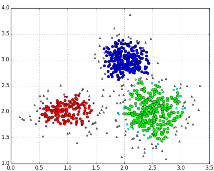
 平均调整兰德指数(aARI)完全指南:聚类与视觉模型评估的核心指标 平均调整兰德指数(Average Adjusted Rand Index, aARI)是机器学习中评估聚类模型与真实标签一致性的重要指标。本文详细解析aARI的计算原理、公式推导及其在语义分割和聚类分析中的实际应用。通过对比准确率、IoU和F1-Score等传统指标,阐述aARI在抗类别不平衡和评估聚类结构方面的独特优势。文章还提供aARI的数学模型、使用场景及与其他指标的对比分析,为研究人员和从业者提供了一套完整的模型评估解决方案,帮助提升模型性能评估的准确性和可靠性。 引言 在计算机视觉和机器学习领域,准确评估模型性能是至关重要的。特别是在语义分割任务中,我们不仅需要知道模型预测的准确性,还需要了解它对不同类别的分割效果。今天,要学习一个强大而实用的评估指标——平均调整兰德指数(Average Adjusted Rand Index, aARI)。 关于指标的结果:平均调整兰德指数的数值越大,代表聚类结果与真实标签的相似度越高,也就是说聚类效果越好。 ARI的提出和改进 兰德指数(Rand Index)最初由William M. Rand在1971年提出,用于衡量两个数据聚类结果的相似性。它的基本思想很直观:比较两个聚类方案中每对数据点的分组情况。 兰德指数是一个用来衡量两个数据聚类结果(比如,一个是算法给出的聚类结果,另一个是数据的真实类别标签)相似度的指标。它通过考虑数据点对(pairs of data points)来计算。具体来说,它衡量的是“一致”决策的比例: 真正例 (True Positives, TP):在真实标签中属于同一类,在聚类结果中也被分到同一簇的点对数量。 真负例 (True Negatives, TN):在真实标签中属于不同类,在聚类结果中也被分到不同簇的点对数量。 公式: $$ \begin{array} { r } { R I = \frac { T P + T N } { T P + F P + F N + T N } } \end{array} $$取值范围:0 到 1 之间。1 表示两个聚类结果完全相同,0 表示完全不同。 兰德指数有一个缺点,即当随机进行聚类时,它的期望值不是一个常数(通常不是0)。即使一个聚类结果是完全随机产生的,RI值也可能看起来还不错,这会让人误判聚类效果。调整兰德指数通过引入一个基于随机情况的期望值来修正这个问题,使得完全随机的聚类结果的ARI期望值为0。 改进版本的计算公式: $$ A R I = \frac { R I - E [ R I ] } { \operatorname* { m a x } ( R I ) - E [ R I ] } $$其中,E[RI] 是在随机分配情况下的兰德指数的期望值。 取值范围:-1 到 1 之间。 1:表示聚类结果与真实标签完全一致,是最好的情况。 接近 0:表示聚类结果与随机分配差不多。 负值:表示聚类结果比随机分配还要差。 平均调整兰德指数 (aARI) 这个指标通常出现在需要多次评估或在不同数据集分区上评估聚类算法性能的场景中,例如: 交叉验证 (Cross-Validation):在进行K折交叉验证时,每一折都会产生一个ARI值。将这K个ARI值取平均,就得到了平均调整兰德指数。 多次重复实验:对于一些带有随机性的聚类算法(如K-Means,其初始中心是随机选择的),为了得到一个稳定且可靠的性能度量,通常会多次运行算法,每次计算一个ARI值,最后取其平均值。 因此,平均调整兰德指数(aARI)就是对多次实验或多个数据集子集上计算出的调整兰德指数(ARI)的平均值。它继承了ARI的所有特性。 aARI vs 其他指标 指标优点缺点适用场景准确率(Accuracy)直观易懂受类别不平衡影响严重类别平衡的简单分类IoU/mIoU考虑重叠区域对小目标不够敏感目标检测、语义分割F1-Score平衡精确率和召回率不考虑聚类结构二分类或多分类aARI考虑聚类结构,抗类别不平衡计算相对复杂语义分割、聚类任务聚类任务图片 此部分内容需要付费后才能阅读 您当前未登录,游客身份购买的内容仅在当前浏览器生效 (7天)。 清除Cookie或更换设备后需重新购买。 为获得永久阅读权限, 建议注册账户 后购买。 支付 0.01 元阅读 请使用支付宝扫描二维码支付 金额:0.01 元 二维码2小时内有效,支付成功后页面将自动刷新 if(typeof payit_generate_qr === "undefined") { function payit_generate_qr(id, url, cid, price) { var container = document.getElementById(id); var qrContainer = container.querySelector(".payit-qrcode-container"); var qrCodeDiv = container.querySelector(".payit-qrcode"); var btn = container.querySelector(".payit-button"); btn.disabled = true; btn.innerText = "二维码生成中..."; var xhr = new XMLHttpRequest(); xhr.open("POST", url, true); xhr.setRequestHeader("Content-Type", "application/x-www-form-urlencoded"); xhr.onreadystatechange = function () { if (xhr.readyState === 4) { if (xhr.status === 200) { try { var res = JSON.parse(xhr.responseText); if(res.code === 0 && res.qr_code) { qrContainer.style.display = "block"; container.querySelector(".payit-mask").style.display = "none"; new QRCode(qrCodeDiv, { text: res.qr_code, width: 150, height: 150 }); payit_check_status(id, "https://www.hubtools.cn/payit/check", res.out_trade_no); } else { alert("二维码生成失败: " + (res.msg || "未知错误")); btn.disabled = false; btn.innerText = "支付 " + price + " 元阅读"; } } catch (e) { alert("从服务器获取数据时出错。"); btn.disabled = false; btn.innerText = "支付 " + price + " 元阅读"; } } else { alert("请求服务器失败。"); btn.disabled = false; btn.innerText = "支付 " + price + " 元阅读"; } } }; xhr.send("cid=" + cid + "&price=" + price); } } if(typeof set_payit_cookie === "undefined") { function set_payit_cookie(name, value, days) { var expires = ""; if (days) { var date = new Date(); date.setTime(date.getTime() + (days*24*60*60*1000)); expires = "; expires=" + date.toUTCString(); } document.cookie = name + "=" + (value || "") + expires + "; path=/"; } } if(typeof payit_check_status === "undefined") { function payit_check_status(id, url, order_id) { var interval = setInterval(function() { var xhr = new XMLHttpRequest(); xhr.open("POST", url, true); xhr.setRequestHeader("Content-Type", "application/x-www-form-urlencoded"); xhr.onreadystatechange = function() { if (xhr.readyState === 4 && xhr.status === 200) { try { var res = JSON.parse(xhr.responseText); if (res.code === 0) { clearInterval(interval); // 如果是游客,前端设置cookie if (res.token) { var cookieName = "payit_cid_" + res.cid; set_payit_cookie(cookieName, res.token, res.expire); } document.getElementById(id).innerHTML = "支付成功,正在刷新页面..."; setTimeout(function() { location.reload(); }, 200); } } catch (e) { /* 支付未成功,不处理 */ } } }; xhr.send("out_trade_no=" + order_id); }, 3000); } } .payit-wrapper { border: 2px dashed #e67e22; background-color: #fdf5ee; padding: 20px; text-align: center; margin: 20px 0; border-radius: 8px; } .payit-wrapper .payit-guest-notice { font-size: 13px; color: #555; background-color: rgba(0,0,0,0.03); border: 1px solid rgba(0,0,0,0.05); padding: 10px; margin: 15px auto; border-radius: 5px; max-width: 95%; line-height: 1.6; } .payit-wrapper .payit-guest-notice p { margin: 5px 0; } .payit-wrapper .payit-guest-notice a { color: #e67e22; font-weight: bold; text-decoration: none; } .payit-wrapper .payit-guest-notice a:hover { text-decoration: underline; } .payit-mask .payit-notice { font-size: 18px; color: #e67e22; font-weight: bold; margin-bottom: 15px; display: flex; align-items: center; justify-content: center; } .payit-mask .payit-button { background-color: #e67e22; color: #ffffff; border: none; padding: 12px 25px; font-size: 16px; cursor: pointer; border-radius: 5px; transition: opacity 0.2s; } .payit-mask .payit-button:hover { opacity: 0.9; } .payit-mask .payit-button:disabled { opacity: 0.6; cursor: not-allowed; } .payit-qrcode-container { color: #333; } .payit-qrcode-container p { margin: 10px 0; } .payit-qrcode { width: 150px; height: 150px; margin: 10px auto; padding: 5px; background: white; border: 1px solid #ddd; border-radius: 3px;}
-
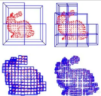
使用 Python NumPy 原生代码实现点云的体素下采样 在 3D 数据处理领域,点云是一种重要的空间信息表示形式,用于捕捉物体和环境的几何形状。然而,点云数据通常非常密集,包含数百万甚至更多的点,这对存储、处理和可视化都带来了挑战。为了解决这个问题,我们需要对点云进行下采样,以减少点的数量,同时尽量保留数据的整体结构。体素下采样(Voxel Downsampling)是一种高效的下采样方法,它通过将点云划分到三维网格(体素)中并对每个体素内的点进行平均来实现这一目标。 什么是体素下采样? 此部分内容需要付费后才能阅读 您当前未登录,游客身份购买的内容仅在当前浏览器生效 (7天)。 清除Cookie或更换设备后需重新购买。 为获得永久阅读权限, 建议注册账户 后购买。 支付 4.99 元阅读 请使用支付宝扫描二维码支付 金额:4.99 元 二维码2小时内有效,支付成功后页面将自动刷新 if(typeof payit_generate_qr === "undefined") { function payit_generate_qr(id, url, cid, price) { var container = document.getElementById(id); var qrContainer = container.querySelector(".payit-qrcode-container"); var qrCodeDiv = container.querySelector(".payit-qrcode"); var btn = container.querySelector(".payit-button"); btn.disabled = true; btn.innerText = "二维码生成中..."; var xhr = new XMLHttpRequest(); xhr.open("POST", url, true); xhr.setRequestHeader("Content-Type", "application/x-www-form-urlencoded"); xhr.onreadystatechange = function () { if (xhr.readyState === 4) { if (xhr.status === 200) { try { var res = JSON.parse(xhr.responseText); if(res.code === 0 && res.qr_code) { qrContainer.style.display = "block"; container.querySelector(".payit-mask").style.display = "none"; new QRCode(qrCodeDiv, { text: res.qr_code, width: 150, height: 150 }); payit_check_status(id, "https://www.hubtools.cn/payit/check", res.out_trade_no); } else { alert("二维码生成失败: " + (res.msg || "未知错误")); btn.disabled = false; btn.innerText = "支付 " + price + " 元阅读"; } } catch (e) { alert("从服务器获取数据时出错。"); btn.disabled = false; btn.innerText = "支付 " + price + " 元阅读"; } } else { alert("请求服务器失败。"); btn.disabled = false; btn.innerText = "支付 " + price + " 元阅读"; } } }; xhr.send("cid=" + cid + "&price=" + price); } } if(typeof set_payit_cookie === "undefined") { function set_payit_cookie(name, value, days) { var expires = ""; if (days) { var date = new Date(); date.setTime(date.getTime() + (days*24*60*60*1000)); expires = "; expires=" + date.toUTCString(); } document.cookie = name + "=" + (value || "") + expires + "; path=/"; } } if(typeof payit_check_status === "undefined") { function payit_check_status(id, url, order_id) { var interval = setInterval(function() { var xhr = new XMLHttpRequest(); xhr.open("POST", url, true); xhr.setRequestHeader("Content-Type", "application/x-www-form-urlencoded"); xhr.onreadystatechange = function() { if (xhr.readyState === 4 && xhr.status === 200) { try { var res = JSON.parse(xhr.responseText); if (res.code === 0) { clearInterval(interval); // 如果是游客,前端设置cookie if (res.token) { var cookieName = "payit_cid_" + res.cid; set_payit_cookie(cookieName, res.token, res.expire); } document.getElementById(id).innerHTML = "支付成功,正在刷新页面..."; setTimeout(function() { location.reload(); }, 200); } } catch (e) { /* 支付未成功,不处理 */ } } }; xhr.send("out_trade_no=" + order_id); }, 3000); } } .payit-wrapper { border: 2px dashed #e67e22; background-color: #fdf5ee; padding: 20px; text-align: center; margin: 20px 0; border-radius: 8px; } .payit-wrapper .payit-guest-notice { font-size: 13px; color: #555; background-color: rgba(0,0,0,0.03); border: 1px solid rgba(0,0,0,0.05); padding: 10px; margin: 15px auto; border-radius: 5px; max-width: 95%; line-height: 1.6; } .payit-wrapper .payit-guest-notice p { margin: 5px 0; } .payit-wrapper .payit-guest-notice a { color: #e67e22; font-weight: bold; text-decoration: none; } .payit-wrapper .payit-guest-notice a:hover { text-decoration: underline; } .payit-mask .payit-notice { font-size: 18px; color: #e67e22; font-weight: bold; margin-bottom: 15px; display: flex; align-items: center; justify-content: center; } .payit-mask .payit-button { background-color: #e67e22; color: #ffffff; border: none; padding: 12px 25px; font-size: 16px; cursor: pointer; border-radius: 5px; transition: opacity 0.2s; } .payit-mask .payit-button:hover { opacity: 0.9; } .payit-mask .payit-button:disabled { opacity: 0.6; cursor: not-allowed; } .payit-qrcode-container { color: #333; } .payit-qrcode-container p { margin: 10px 0; } .payit-qrcode { width: 150px; height: 150px; margin: 10px auto; padding: 5px; background: white; border: 1px solid #ddd; border-radius: 3px;} 代码实现 以下是一个完整的 Python 脚本,使用 NumPy 实现点云的体素下采样。代码简洁高效,适用于大多数基本的点云处理需求。 import numpy as np from collections import defaultdict def read_point_cloud(file_path): """读取点云文件,假设每行是一个点的xyz坐标,可能包含其他属性""" points = [] with open(file_path, 'r') as f: for line in f: parts = line.strip().split() if len(parts) >= 3: # 至少包含xyz三个坐标 x, y, z = map(float, parts[:3]) points.append([x, y, z]) return np.array(points) def voxel_downsample(points, voxel_size): """体素下采样""" # 创建体素网格 voxel_grid = defaultdict(list) # 计算每个点所在的体素 for point in points: voxel_coord = tuple((point // voxel_size).astype(int)) voxel_grid[voxel_coord].append(point) # 对每个体素内的点取平均 downsampled_points = [] for voxel_coord, voxel_points in voxel_grid.items(): if voxel_points: avg_point = np.mean(voxel_points, axis=0) downsampled_points.append(avg_point) return np.array(downsampled_points) def write_point_cloud(file_path, points): """将点云写入文件""" with open(file_path, 'w') as f: for point in points: f.write(f"{point[0]} {point[1]} {point[2]}\n") def main(): # 配置参数 input_file = "test1_pointcloud - Cloud.subsampled.txt" # 输入点云文件 output_file = "downsampled_test1_pointcloud - Cloud.subsampled.txt" # 输出点云文件 voxel_size = 1.2 # 体素大小,根据你的点云尺度调整 # 读取点云 points = read_point_cloud(input_file) print(f"原始点云数量: {len(points)}") # 体素下采样 downsampled_points = voxel_downsample(points, voxel_size) print(f"下采样后点云数量: {len(downsampled_points)}") # 保存下采样后的点云 write_point_cloud(output_file, downsampled_points) print(f"下采样后的点云已保存到: {output_file}") if __name__ == "__main__": main()体素大小的选择 体素大小(voxel_size)是下采样的关键参数,直接影响结果: 较大的体素大小:会导致更激进的下采样,点数减少更多,但可能会丢失细节。 较小的体素大小:保留更多细节,但下采样后的点云仍然较大。 选择合适的体素大小需要根据点云的尺度以及应用需求。例如,对于建筑扫描,1 厘米的体素大小可能合适;而对于室外大场景,1 米的体素大小可能更适合。 效果展示 左边是原始的点云,右边是体素下采样之后的点云。 下采样前后的对比图片
-
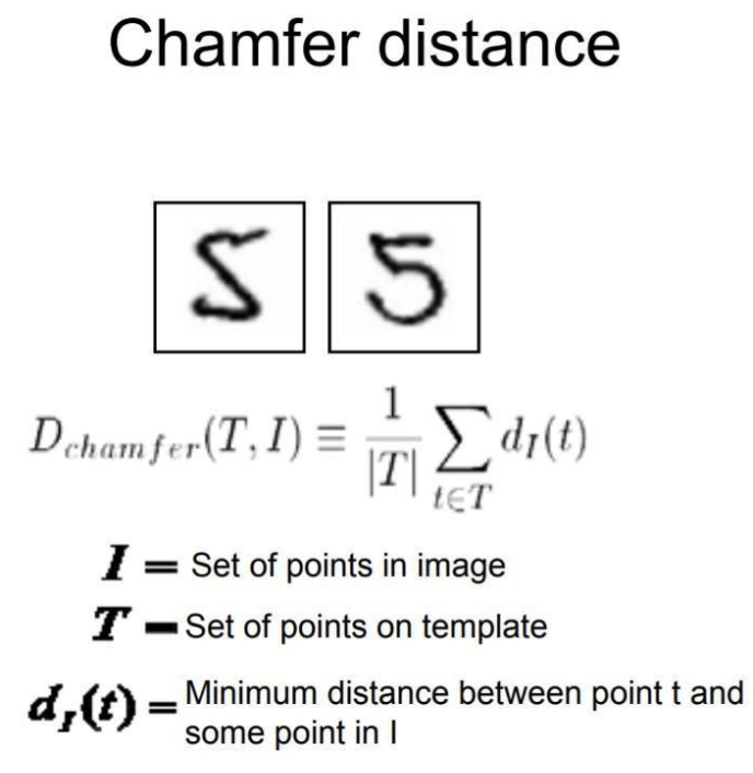
Python 实现 Chamfer 距离:点云相似性度量原理、应用与代码指南 Chamfer 距离(Chamfer Distance, CD)是一种经典的点云相似性度量,广泛用于三维点云完成、配准、模型检索,以及深度学习中的损失函数和评估指标。本文首先介绍 Chamfer 距离的数学定义与变体,包括普通与归一化形式;接着梳理其在点云处理、计算机视觉与机器学习中的典型应用;最后提供两种基于 Python 的实现示例——纯 NumPy 直观版与 SciPy KD-Tree 加速版,帮助开发者快速上手并根据需求优化性能。 1. Chamfer 距离简介 Chamfer 距离(Chamfer Distance, CD)是一种用于评估两组离散点云相似性的“最近邻”度量。它通过计算每个点到另一组点集中最近点的距离之和(或平均),从双向角度量化两点云的重叠与对齐程度。 数学定义(平方欧氏距离) $$ \mathrm{CD}(P, Q) = \sum_{p\in P} \min_{q\in Q} \|p - q\|_2^2 + \sum_{q\in Q} \min_{p\in P} \|q - p\|_2^2 $$ 可选欧氏距离形式 $$ \mathrm{CD}(P, Q) = \sum_{p\in P} \min_{q\in Q} \|p - q\|_2 + \sum_{q\in Q} \min_{p\in P} \|q - p\|_2 $$ 归一化 Chamfer 距离 $$ \mathrm{CD}_{\mathrm{norm}}(P, Q) = \frac{1}{|P|}\sum_{p\in P}\min_{q\in Q}\|p-q\|_2^2 + \frac{1}{|Q|}\sum_{q\in Q}\min_{p\in P}\|q-p\|_2^2 $$ 度量灵活性 可以根据任务需求选择欧氏距离、曼哈顿距离,甚至双曲距离(HyperCD)等。 2. Chamfer 距离的主要应用 三维点云处理 点云完成:作为损失函数与评估指标,量化预测点云与真实点云之间的形状差异; 点云配准:度量不同扫描或模型的对齐质量; 三维模型检索:在数据库中检索形状相似的模型。 计算机视觉 形状匹配与物体检测:基于 Chamfer 系统与定向 Chamfer 距离(OCD)的模板匹配; 图像配准:通过边缘或轮廓对齐多源影像,应用于医学成像与遥感。 机器学习 深度学习损失:点云生成、重建等模型训练的可微距离函数; 评估指标:量化模型输出与真实值之间的几何相似性。 3. 优势与局限 优势局限计算效率高((O(mn)),可用 KD-Tree 优化)对离群点敏感,易受极端偏差影响灵活性强,支持不同点数对局部密度差异不敏感,可能导致错配对轻微形变与位置偏移具有鲁棒性原始定义非对称,需双向求和或归一化以保证对称性相较于 Earth Mover’s Distance (EMD) 和 Hausdorff 距离,Chamfer 距离在实时或大规模场景下更具实用性,但需针对噪声与密度分布设计相应改进。 4. Chamfer 距离 Python 实现 (1)纯 NumPy 实现(直观版) import numpy as np def chamfer_distance_naive(P: np.ndarray, Q: np.ndarray, squared: bool = True) -> float: """ 计算点云 P, Q 之间的 Chamfer 距离(平方或开方形式)。 P: (m, d), Q: (n, d) """ dist_pq = [] for p in P: dists = np.linalg.norm(Q - p, axis=1) dist_pq.append(dists.min() if not squared else (dists**2).min()) dist_qp = [] for q in Q: dists = np.linalg.norm(P - q, axis=1) dist_qp.append(dists.min() if not squared else (dists**2).min()) return np.sum(dist_pq) + np.sum(dist_qp) # 示例测试 P = np.random.rand(100, 3) Q = np.random.rand(120, 3) print("Chamfer 距离(纯 NumPy,平方):", chamfer_distance_naive(P, Q, squared=True))(2)KD-Tree 加速实现(高效版) import numpy as np from scipy.spatial import cKDTree def chamfer_distance_kdtree(P: np.ndarray, Q: np.ndarray, normalized: bool = False) -> float: """ 基于 cKDTree 的 Chamfer 距离计算,默认使用平方欧氏距离。 """ tree_P = cKDTree(P) tree_Q = cKDTree(Q) dist_pq, _ = tree_Q.query(P, k=1, n_jobs=-1) dist_qp, _ = tree_P.query(Q, k=1, n_jobs=-1) cd_val = np.sum(dist_pq**2) + np.sum(dist_qp**2) if normalized: cd_val = cd_val / len(P) + cd_val / len(Q) return cd_val # 示例测试 print("Chamfer 距离(KD-Tree,归一化):", chamfer_distance_kdtree(P, Q, normalized=True))5. 小结与展望 Chamfer 距离以其高效、灵活、鲁棒的特点,已成为点云与形状匹配领域的常用度量。然而,其对离群点与密度变化的敏感性,也催生了多种变体和改进方向: 鲁棒性增强:引入加权机制或密度补偿,降低离群点影响; 全局与局部融合:结合 EMD、谱距离等,提升整体结构一致性; 跨模态扩展:应用于 LiDAR 与 RGB-D 融合、医学影像配准等新场景。 Chamfer 距离图片
-
-
Python+蚁群算法实战:医院科室智能调度等待时间优化系统开发(附完整开源代码) 本文针对三甲医院多科室体检排队效率痛点,基于生物启发算法提出创新解决方案。通过将7大检查科室建模为动态TSP问题,利用Python构建多线程优先队列仿真系统,结合蚁群算法的信息素动态更新机制,实现科室访问路径智能优化。实验数据显示,该方案较传统随机排队模式减少患者总等待时长22.6%,科室间转移效率提升35%,算法在50次迭代内快速收敛。文中完整公开含多服务台调度、Matplotlib热力图可视化等核心模块的代码实现,为医疗资源优化、智能医院建设提供可直接复用的开源解决方案,特别适合AI医疗、运筹优化等领域的开发者参考学习。 在现代医院门诊流程中,患者往往需要在多个检查科室之间来回奔波,面临长时间的排队等待。以某医院为例,患者通常需要完成7项检查:抽血室(5分钟,2个服务台)、B超室(20分钟)、眼科(5分钟)、内科(10分钟)、外科(15分钟)、心电图(10分钟)和身高体重测量(5分钟)。每位患者平均每2分钟到达医院(即30人/小时),在科室间转移还需额外花费2分钟时间。 这种复杂的排队系统导致患者总等待时间过长,不仅影响就医体验,也降低了医院运营效率。传统的人工调度或随机排队方式难以实现最优的资源配置,因此需要一种智能化的解决方案来优化患者的科室访问顺序,从而显著减少总等待时间。 解决思路 针对这一复杂的排队优化问题,我们采用了受自然界蚂蚁觅食行为启发的蚁群算法。该算法的核心思想是通过模拟蚂蚁群体在寻找食物过程中释放信息素的行为,逐步发现最优的路径选择策略。 具体实施中,我们将每位患者视为一个需要完成所有检查的"旅行者",各科室则是必须访问的"城市"。算法通过以下机制实现优化: 信息素引导:记录历史优质解决方案中科室间的转移偏好 启发式信息:考虑各科室的平均检查时间(时间越短优先级越高) 概率选择:平衡已知最优路径探索与新路径开发 动态更新:根据解决方案质量调整信息素浓度 系统特别考虑了不同科室服务台数量的差异(如抽血室有2个服务台),使用优先队列(最小堆)精确模拟多服务台排队场景,确保等待时间计算的准确性。 验证方法 为验证算法的有效性,我们设计了科学的对比实验: 基准测试:采用完全随机的科室访问顺序作为对比基准 评价指标:计算所有患者的总等待时间,包括: 在各科室外的排队等待时间 科室间转移的固定时间(2分钟/次) 优化率计算:(随机方案耗时-优化方案耗时)/随机方案耗时×100% 实践代码 由于使用了一些外部库,需要使用下面的命令进行安装: pip install matplotlib seaborn numpy 当然在国内可以使用更快的清华镜像源: pip install matplotlib seaborn numpy -i https://mirrors.tuna.tsinghua.edu.cn/pypi/web/simple以下是完整的代码: import random import heapq import matplotlib.pyplot as plt import seaborn as sns import numpy as np from matplotlib import font_manager # 设置中文字体 try: plt.rcParams['font.sans-serif'] = ['Microsoft YaHei'] # Windows系统常用 plt.rcParams['axes.unicode_minus'] = False except: try: plt.rcParams['font.sans-serif'] = ['SimHei'] # 备选方案 plt.rcParams['axes.unicode_minus'] = False except: print("无法设置中文字体,将使用默认字体") # 科室信息 departments = [ {'name': '抽血室', 'time': 5, 'servers': 2}, {'name': 'B超室', 'time': 20, 'servers': 1}, {'name': '眼科', 'time': 5, 'servers': 1}, {'name': '内科', 'time': 10, 'servers': 1}, {'name': '外科', 'time': 15, 'servers': 1}, {'name': '心电图室', 'time': 10, 'servers': 1}, {'name': '身高体重', 'time': 5, 'servers': 1}, ] dept_names = [dept['name'] for dept in departments] num_departments = len(departments) dept_times = [dept['time'] for dept in departments] eta = [1.0 / dept['time'] for dept in departments] # 启发式信息 # 算法参数 alpha = 1 # 信息素权重 beta = 2 # 启发式信息权重 rho = 0.1 # 信息素蒸发率 Q = 1000.0 # 信息素增强系数 num_ants = 10 # 蚂蚁数量 iterations = 50 # 迭代次数 num_patients = 30 # 患者数量 # 生成到达时间(每2分钟一个患者) arrival_times = [i * 2 for i in range(num_patients)] # 初始化信息素矩阵 tau = [[1.0 for _ in range(num_departments)] for _ in range(num_departments)] def roulette_wheel_selection(probabilities): """轮盘赌选择算法""" r = random.uniform(0, sum(p for _, p in probabilities)) cumulative = 0 for j, p in probabilities: cumulative += p if cumulative >= r: return j return probabilities[-1][0] def generate_path(tau, eta): """生成单个患者的科室访问路径""" path = [] unvisited = set(range(num_departments)) # 随机选择起始科室 current = random.choice(list(unvisited)) path.append(current) unvisited.remove(current) while unvisited: probabilities = [] total = 0.0 for j in unvisited: pheromone = tau[current][j] heuristic = eta[j] prob = (pheromone ** alpha) * (heuristic ** beta) probabilities.append((j, prob)) total += prob if total == 0: # 处理零概率情况 j = random.choice(list(unvisited)) else: probabilities = [(j, p / total) for j, p in probabilities] j = roulette_wheel_selection(probabilities) path.append(j) unvisited.remove(j) current = j return path def evaluate_solution(patients_paths): """评估解决方案的总等待时间""" # 初始化科室服务台(使用最小堆) queues = [] for dept in departments: servers = [0] * dept['servers'] heapq.heapify(servers) queues.append(servers.copy()) total_wait = 0 for pid in range(num_patients): path = patients_paths[pid] arrival = arrival_times[pid] current_time = arrival for i, dept in enumerate(path): # 计算到达时间 if i == 0: dept_arrival = arrival else: dept_arrival = current_time + 2 # 转移时间 # 获取服务台 queue = queues[dept] available_time = heapq.heappop(queue) # 计算等待时间 wait_time = max(0, available_time - dept_arrival) total_wait += wait_time # 更新服务台时间 start_time = max(dept_arrival, available_time) end_time = start_time + departments[dept]['time'] heapq.heappush(queue, end_time) current_time = end_time # 添加转移时间 total_wait += 2 * (len(path) - 1) return total_wait # 运行蚁群算法 best_solution = None best_cost = float('inf') best_costs_history = [] # 记录每次迭代的最佳成本 for iteration in range(iterations): solutions = [] for _ in range(num_ants): # 生成蚂蚁解决方案 paths = [generate_path(tau, eta) for _ in range(num_patients)] cost = evaluate_solution(paths) solutions.append((cost, paths)) # 更新全局最优 if cost < best_cost: best_cost = cost best_solution = paths best_costs_history.append(best_cost) print(f"迭代次数 {iteration + 1}: 当前最优等待时间 {best_cost} 分钟") # 信息素蒸发 for i in range(num_departments): for j in range(num_departments): tau[i][j] *= (1 - rho) # 信息素增强 for cost, paths in solutions: if cost == best_cost: for path in paths: for k in range(len(path) - 1): i = path[k] j = path[k + 1] tau[i][j] += Q / cost # 随机解决方案对比 random_paths = [random.sample(range(num_departments), num_departments) for _ in range(num_patients)] random_cost = evaluate_solution(random_paths) improvement = (random_cost - best_cost) / random_cost * 100 # 1. 优化过程可视化 plt.figure(figsize=(12, 5)) plt.subplot(1, 2, 1) plt.plot(range(1, iterations + 1), best_costs_history, 'b-', linewidth=2) plt.title('蚁群算法优化过程') plt.xlabel('迭代次数') plt.ylabel('总等待时间(分钟)') plt.grid(True) # 标记最优解 optimal_iter = best_costs_history.index(min(best_costs_history)) + 1 optimal_cost = min(best_costs_history) plt.scatter(optimal_iter, optimal_cost, color='red', s=100, label=f'最优解: {optimal_cost} 分钟 (第{optimal_iter}次迭代)') # 添加随机方案参考线 plt.axhline(y=random_cost, color='g', linestyle='--', label=f'随机方案: {random_cost} 分钟') plt.legend() # 2. 科室访问热力图 plt.subplot(1, 2, 2) transfer_matrix = np.zeros((num_departments, num_departments)) for path in best_solution: for k in range(len(path) - 1): i = path[k] j = path[k + 1] transfer_matrix[i][j] += 1 sns.heatmap(transfer_matrix, annot=True, fmt='.0f', cmap='YlOrRd', xticklabels=dept_names, yticklabels=dept_names) plt.title('科室间转移频率热力图') plt.xlabel('目标科室') plt.ylabel('来源科室') plt.tight_layout() plt.show() # 打印最终结果 print("\n===== 最终优化结果 =====") print(f"随机排队总等待时间: {random_cost} 分钟") print(f"优化后总等待时间: {best_cost} 分钟") print(f"优化率: {improvement:.2f}%") if improvement >= 20: print("优化目标达成 (优化率≥20%)") else: print("优化目标未达成")关于代码的一些配置如下。首先是根据题意进行科室信息的配置: 科室信息的配置图片 然后就是算法的基本参数配置: 基本参数配置图片 代码一次运行效果如下: 运行效果图片 热力图图片 通过可视化,可以直观地展示: 算法收敛过程 最优解出现的位置 患者在不同科室间的流动模式 优化前后的对比效果 科室访问热力图的作用: 使用seaborn绘制科室间转移频率的热力图 横纵坐标标注科室名称 颜色深浅表示转移频率高低